This is a ‘write it down before I forget’ post. I have shared it in case anyone else is overcome by a sense of existential dread at having to use Bionumerics.

Minimum spanning trees are a nice way to present data when you want to express the relationship between different genotypes you have observed and the number of occurrences of each genotype.

There are a couple of ways of doing them (including Joao Carrico’s Phyloviz). However, lab scientists at PHE  use Bionumerics to store/analyse data and it outputs nice plots (eventually!). This blog post explains how to use bionumerics to construct minimum spanning trees. The data set is a collection of over 100 shiga toxin 1 (stx) gene sequences. Before I started, I made a pseudo-sequence of the 16 variant positions in my stx alignment. Then…

1. In excel, get variant positions, replace the A, T, C, G with 1-4, with strain ids and variant number as column headings. Select data and assign to ‘data’ variable in top left corner. save as a .xls file (see fig 1).
2. In bionumerics, create a new local database. Then follow the below steps, most refer to a selection from a drop down menu.
3. Database -> ODBC link -> configure external -> select -> machine data source -> excel files -> point to data.xls -> in database table put ‘data’ -> Link the ‘stx’ to Key
4. Database -> ODBC link -> copy data from external database
5. Create new experiment -> new character type -> numerical values
6. Double click on created character type -> file -> import from external database -> select variant columns -> create character -> ok
7. Double click on created character type again -> file -> import from external database
8. In main screen right click on header -> add new information field -> give name -> right click on new information field -> download field from external database -> select correct name
9. edit -> select all -> create new comparison -> select stx1a from experiments (top left) -> right click on colour in information fields -> create groups from database field -> create groups alphabetically
10. advanced clustering -> MST -> bingo! Figure 2. Reward your self with a stiff drink.

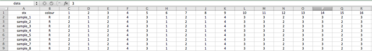Figure 1: expected data format

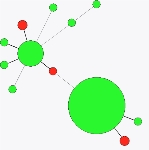
Figure 2: Expected output