I attended the GenEpi Day at London School of Hygeine and Tropical Medicine on Wednesday (would highly recommend attending if they run it again). For me, there were a couple of highlights – Ed Feil’s talk and the use of R for sequence analysis. This post will be about the use of R for sequence analysis.

I do most of my basic sequence exploration in viewers like Mega or BioEdit and  anything more analytical in Python. On the course there was a session on reconstructing disease outbreaks from genome sequences led by Thibaut Jombart, who has written various R packages for this sort of thing.

While the outbreak analysis stuff later in the tutorial was cool, I also found the basic data exploration steps very interesting. The first thing we did was load in a sequence alignment and examine the distribution of SNPs along the length of the sequence. I thought this could be useful for a problem I have had previously – i.e. identifying characteristic SNPs between groups of sequences (e.g. toxin subtypes).

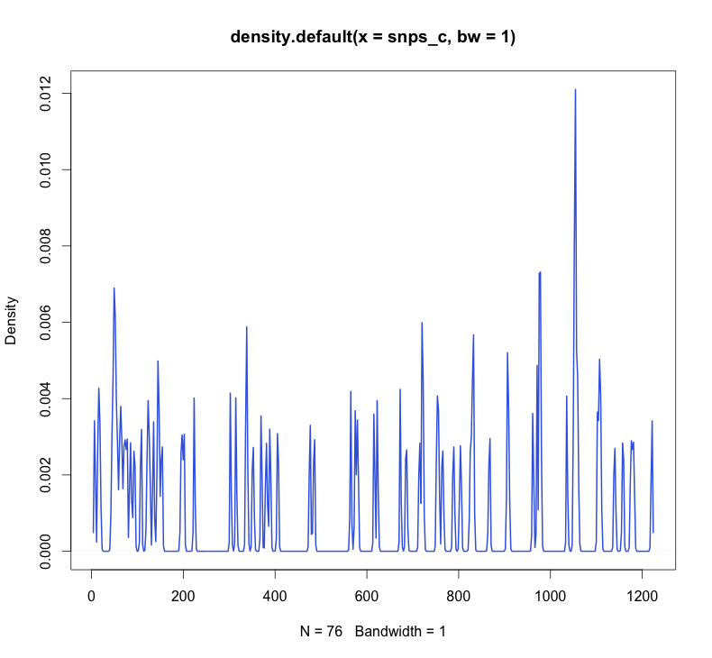
The above figure shows the distribution of SNPs along an alignment of shiga toxin 2c (stx2c) sequences from a recent paper (the N = 76 refers to the number of SNPs in that sequence). If I’m 100% honest, I’m not sure what the height of the plot indicates – probably the number of SNPs within a certain window. It would be cool if the height was proportional to the number of variants at a position, but it doesn’t appear to be. Essentially, the take home from this is that there is quite a lot of differences between different stx2c sequences.

That is quite useful, but what problem does it help us solve? Well, in this case I’m looking for SNPs that differentiate between stx2a and stx2c with 100% specificity and sensitivity. I plotted three plots on the same axis – the SNPs between the 21 stx2a sequences, the SNPs between the 18 stx2c sequences and the SNPs when both subtypes (39 sequences total) were compared.

This figure (full size version available on Figshare here) has the stx2a SNPs (blue), stx2c SNPs (red) and the SNPs when stx2a and 2c were analysed (yellow).

Any SNPs that differentiate cleanly between subtypes will obviously not show up as SNPs in either the stx2a or stx2c plots. However, they will show up as SNPs when we compare stx2a with stx2c. Therefore we are looking for positions that are only covered by yellow peaks. There was one area of the gene where this happened (highlighted with black arrow in figure above).

Then, when we go back to Mega, we can see that these are the only positions that vary with 100% sensitivity between stx2a and stx2c (there really aren’t any others, this gene is a bit of a nightmare!).

This is just a toy example really, but, considering that it only takes a few lines of R (3 to load and plot each alignment!) to generate this I will definitely be exploring R sequence analysis options in the future. A great place to get started on that is http://adegenet.r-forge.r-project.org/. Details of how to perform this analysis can be found on that site if you navigate to the Documents page, then scroll down to ‘GenEpi workshop’ and read through the practical (all GPL 2).

If you have any problems or want more info, comment below or tweet me.