Or, how I failed advanced file copying.

TL:DR?

• Phylogenetic trees can be hard to interpret – use bootstraps to help!
• Low coverage in one strain or having an outlier can screw with your tree
• Including positions that have been ignored due to low quality in some of your strains can be useful (i.e. use RAxML and include Ns in your alignment)
• cat with caution

We need to start training clinical microbiologists in phylogenetic tree interpretation. You can have the slick-est, point and click-iest pipeline to go from fastqs -> phylogenetic tree, but if the scientist generating the tree doesn’t know their tips from their roots, there isn’t much point (or click).

As someone who has only moved into phylogenetics in the last year or two, I can definitely empathise with these people. I had a weird tree yesterday and thought I would jot down a few points on how to trouble shoot a troublesome tree. I’m going to give a bit of theory, then some practical advice. Toward the end it descends into what we do at PHE, but hopefully it will be useful for people grappling with similar issues. I’m assuming you are using FastTree to generate trees and FigTree to visualise.

The first question is, how do I tell that I have a dodgy tree? One of the easiest ways to tell this is to look at the bootstrap values. This is essentially testing whether your whole dataset is supporting your tree, or whether if you remove a bit of your data, you get a very different tree. A rule of thumb is that bootstrap values < 0.8 are a bit weak. In practice, to look at the bootstraps FastTree generates (which are optimised for speed rather than accuracy), when you load your tree into FigTree, it will tell you that your nodes/branches are labelled and ask you to select a name. Enter whatever you like, then in FigTree tick the Node Labels box and then choose to display whatever you put into node label box when you opened your tree. You should see a number on each node, hopefully, close to 1.

So, what happened yesterday? I had a nice tree of a clonal complex of Salmonella, then I added 100 more strains and the tree structure went doolally.

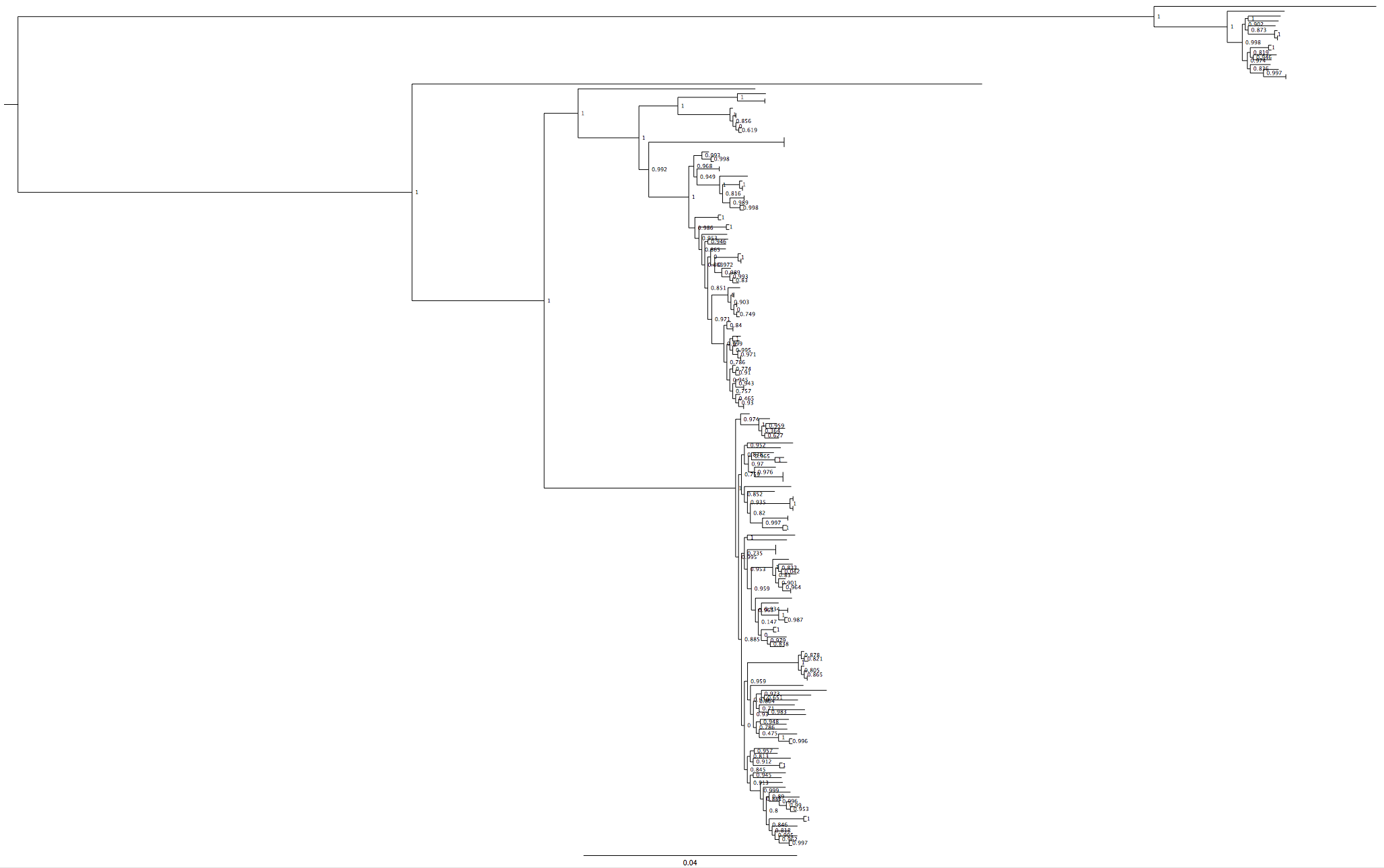
Fig 1: Before new strains

 

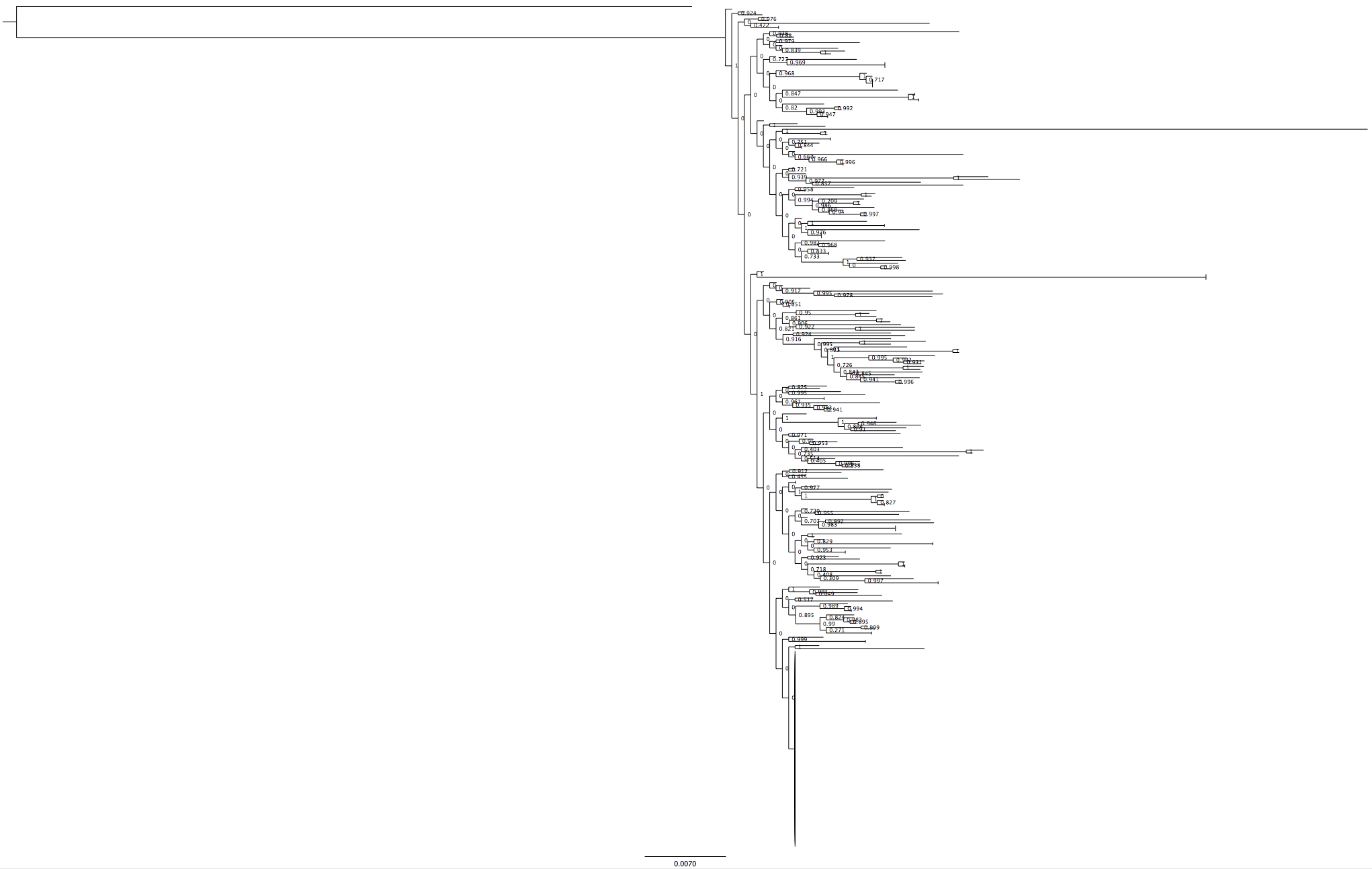
Fig 2: After new strains – that big line at the bottom is not an outbreak.

The structure of the trees in Fig1 and Fig2 are fundamentally different. That is probably easiest to see if you look at the group of strains at the ‘top’ of figure 1, then look for the similar group in Fig2 – it isn’t there, there is only a single strain on the branch at the top of the tree. Also, a diverse group of strains has collapsed into a single line in Fig2.

How can I tell that those strains are diverse and not actually an outbreak? I could look at my original tree, which contains some of these strains and see that in the original, these strains are on divergent branches. But what if I didn’t have an original tree to compare with?

Whenever you have an odd looking tree, some of the things you should look at are:

• The depth of coverage of the new strains, if this is low, you will have a higher number of ignored positions and your core genome will be smaller, which will effect the tree.
• The number of variants in each strain, if you have a massive outlier, it indicates that one of your samples is unrelated to the others, which will decrease the size of your core genome. This should be obvious from the tree.

These common problems were not happening in this case, so what was going on?

You can use a couple of things that we (PHE/Gastro) will output with each tree. These are specific to our pipeline at PHE, but you could (and should?) generate something similar for your own trees. The first thing to look at is the ‘SNP address’, which will hopefully be on your tree (if you work in the gastro department of PHE) as default (we haven’t done that bit of the pipeline yet). This is a numeric representation of hierarchical (single linkage) clusters for a series of specified SNP distances. Clear? Perhaps an example will help. If the series of specified SNP distances was 50:25:10:5, each strain will be assigned to a 5, 10, 25 and 50 SNP cluster, each of which will be given an identifying number. If two strains are in the same 50 SNP cluster, they will share the first number of their SNP address, and so on. For example:

Strain 1 – 3.19.7.44

Strain 2 – 3.19.7.17

Strain 3 – 3.4.35.19

All these strains are in the same 50 SNP cluster (i.e. 50 SNP cluster 3). s1 (strain 1) and s2 are in the same 25 SNP cluster (19), while s3 is at least 25 SNPs distant from any strain (i.e. single linkage) in 25 SNP cluster 19. s1 and s2 are in the same 10 SNP cluster, but different 5 SNP clusters. One of the important things about the SNP address is that it is generated from a distance matrix that is calculated based on pairwise comparison on the genomes, rather than just the core genome. If it was just generated on the core genome, it would more or less exactly follow the tree structure, which wouldn’t be very useful. But, since it is full pairwise comparison, it tells us whether those two strains that look very similar on the tree are similar when we compare their full genomes (within the confines of the reference mapping paradigm).

Well, that was a diverting detour into the mind of Tim, but how does it help in this situation? If I generate the clustering based on the strains in fig 1, we get pretty much what is expected, most 5 SNP clusters have only a single strain in, or a small group (< 5 strains). When I generated the SNP address for the strains in fig2, one of the 5 SNP clusters has over 100 strains in, these are spread throughout the tree but are always close to the root of the bottom branch. Essentially, my clustering has ‘collapsed’, and instead of being nice and ‘branchy’ as in figure 1, it has swelled into an amorphous lump.

Well, this was most upsetting.

It was solved by using a RAxML tree via the CIPRES cluster (a supercomputer with phylogenetic software installed on that you can run compute-intensive jobs like RAxML on, for free!). RAxML is a tree-building program that is optimised for accuracy rather than speed. One of it’s advantages is that it can use positions which aren’t present in all the samples in your alignment to inform the tree structure.

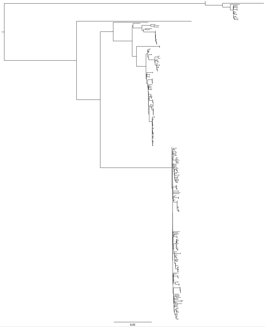
Fig 3: RAxML tree (LB16) that included my troublesome new strains, the structure returns

The fact that the tree structure returned when we included positions that were not present at high quality (i.e. that were being ignored) in all strains indicates that something in the genome was not right. Interestingly, one group of strains in the RAxML tree were still very close to the root of the bottom branch. Tim noticed that many of these strains were labelled ‘cat’.

For some strains, I concatenated two replicates of the same sample together, in order to obtain sufficient depth of coverage for high quality analysis. If I had concatenated two divergent samples together then all the SNPs that differentiated those strains would suddenly become heterozygous positions and would be ignored. This wouldn’t lead to a big leap in the number of ignored positions, as it is only the variants (of which there are a few thousand total) that would be added, and there are hundreds of thousands of ignored positions already.

I removed the concatenated samples, generated the SNP sequence and made a FastTree tree.

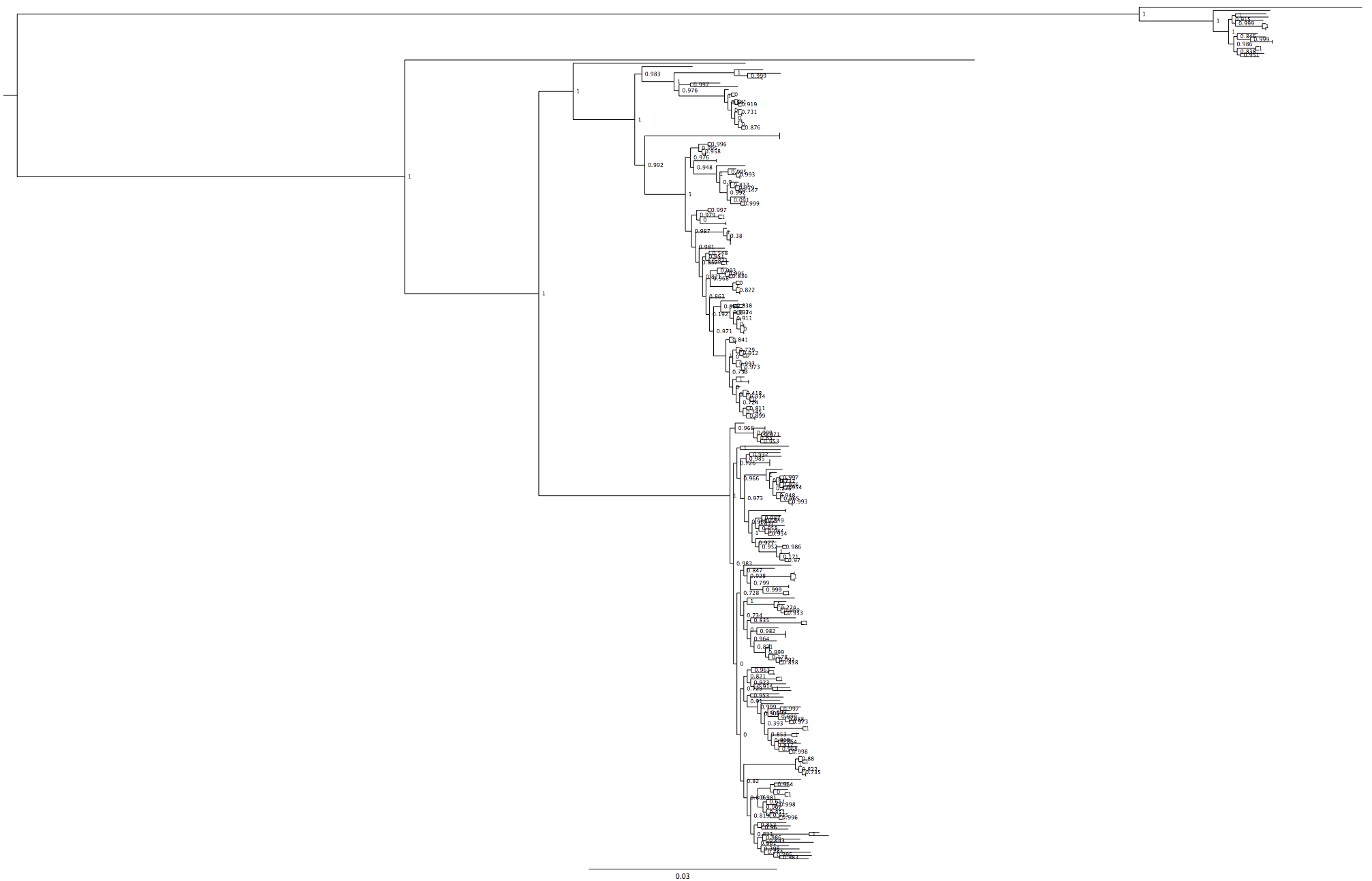
Fig4: Ta da! Correct tree structure, including the new strains (not the ‘cat’ strains)